Binary Classification with Artificial Neural Networks

Introduction:

This report aims to solve a binary classification task using python’s keras library to implement a feedforward artificial neural network. The dataset used is from the finance sector and contains variables that aim to predict a binary outcome. 

ANNs are computational models inspired by the human brains, they consist of interconnected nodes that are organised into layers and each node processes input data and passes it to an activation function for an output. 

This project focuses on exploring different hidden layers and hyperparameters necessary for the model’s optimal performance, providing a rationale for choosing each configuration and comparing performance using different metrics. 

Observing the Dataset:

I started by importing the relevant modules needed for this classification. 

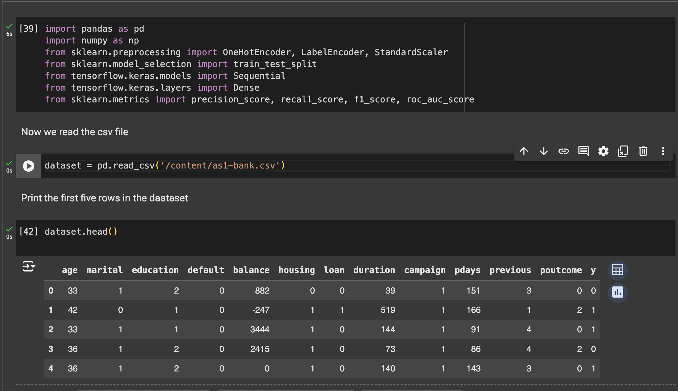
Then I read the dataset using the pandas dataframe.  After that, I decided to inspect the dataset to have a better understanding of the variables. 

The dataset contains 7843 rows, 14 columns including 1 target variable. These features contain various financial metrics and market indicators. I also observed that there are no missing values and no duplicates. Most of the columns seem to be relevant except for the contact variable which I excluded from the dataset.

My reason for not removing columns such as pdays, duration, day, month previous, p-outcome and marital status is because they seem relevant. For instance, regular campaigns might have a positive effect on married people than single ones. Also, according to (Williams, 2023), “there are actually certain months or seasons that are better for certain purchases”. The month and days of the week influences marketing strategies as clients tend to be more relaxed (hence more purchases) on weekends rather than weekdays.

Data Pre-processing

Separating Independent Variables from the Target Variable.

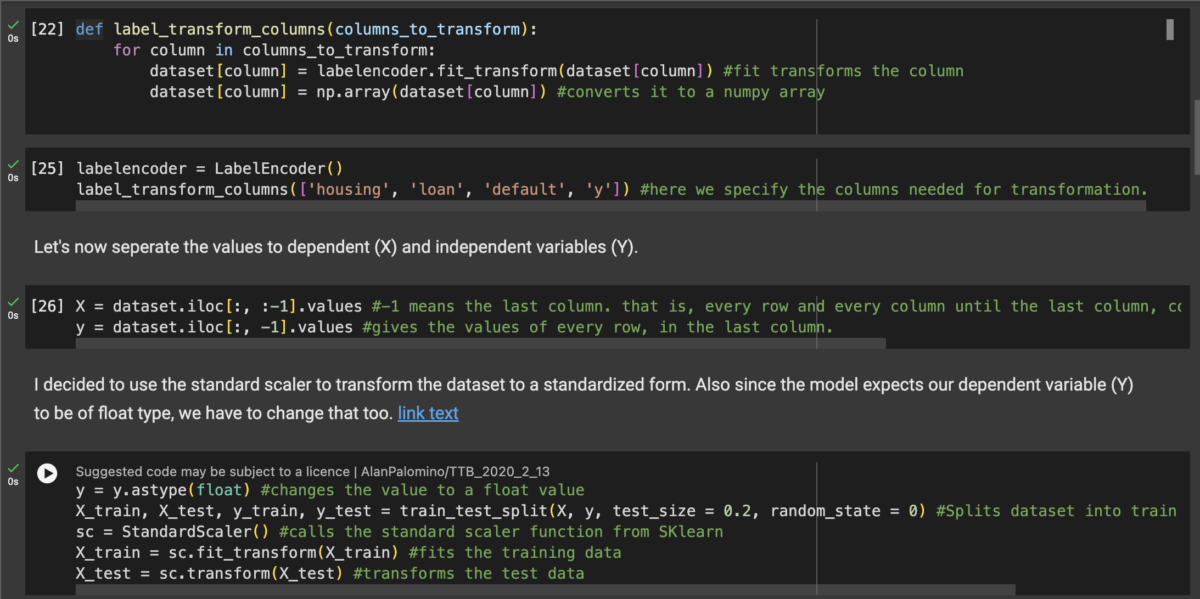
Our target variable (the dependent variable) is the column “y”, which is categorical and describes if a client has subscribed to a term deposit or not. Other columns in the dataset will be the independent variables X. 

Encoding Categorical Variables 

There are 4 categorical variables in this dataset that are not yet transformed. I used label encoding to encode values of the 4 variables to 0 and 1.

Train-Test Split

I imported the train_test_split function from sklearn.model_selection which enabled me to split the data into training and testing sets for both the  independent and output variables. The split test-size will be 0.3, meaning 70 percent for training and 30% for testing. 

Feature Scaling/Standardization

The StandardScaler() from sklearn.preprocessing import StandardScaler was used to scale the values of the training and testing set of the independent variables, that is the predictors. Standardisation ensures that all features are on a similar scale, with a mean of 0 and a standard deviation of 1.  I used standardisation because is important for neural networks as it improves the performance, speed, and convergence of models during training.  The target variable was not standardised as it already has values of 0 and 1. According to (Simon Benavides Pinjosovsky, 2023) “to prevent any information leakage from the testing set into the training set”, normalisation and standardisation should be done after splitting the dataset into testing and training sets.

Architecture of the Feed-Forward Model

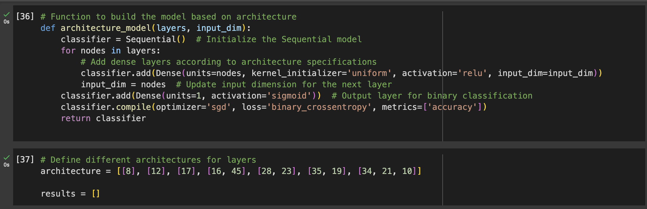
The Keras library was used to build and train a series of ANN architectures which were tested to determine the optimal configuration. The architectures varied in the number of hidden layers and the number of nodes per layer. The Stochastic Gradient Descent was the default optimiser. All models used the ReLU activation function for hidden layers and the sigmoid activation function for the output layer.

To build the architecture of this feed forward neural network, I tested a series of ANN architectures for optimal performance. It consisted of single, double, and triple hidden layers.

The layers used are:

• One hidden layer –  [8], [12], and [17].
• 3 different two hidden layers –  [16, 45], [28, 23], and [35, 19]
• Three hidden layers [34, 21, 10]

For each layer in this architecture, the model is fitted with a batch size of 10, validation split of 0.2 for 50 epochs. The create_model function takes the input dimension, layers of the architecture, activation function and the output activation function as arguments.

Compiling the model: With every layer, I used the sigmoid activation function, this function “maps most inputs to be either very close to zero or very close to one, while still being differentiable.” (Topper, 2023). The model is then compiled using ‘sgd’ as the optimizer and binary_crossentropy to determine the loss. 

The number of hidden layers and nodes were influenced by several factors including the risk of overfitting, the type of model and the nature of this dataset. These were continually adjusted to monitor the changes for optimal performance. Also, Increasing the number of layers enabled the model to learn the representation of variables while improving its generalisability on unseen data. This architecture was continually adjusted to monitor changes for optimal performance.

Reasons Behind My Decision

More nodes in a layer can capture more complex features, especially for complex tasks such as image recognition. Adding more layers in the network can allow it to learn more abstract representations.  Additionally, the number of neurons in each hidden layer were fine-tuned to inspect the accuracy of the models, with the aim to prevent underfitting and overfitting. Relu was used as the preferred activation function for the hidden layer as it introduces non-linearity to the model, allowing it to learn complex features between variables. According to (Aswini, 2023) “An advantage of ReLU, despite avoiding the vanishing gradients problem, is that it has a much lower run time max(0,f) and runs much faster than any sigmoid function.”.

In order to minimise the loss function during training, Stochastic Gradient Descent was used because of its effectiveness and simplicity in learning patterns. The complexity and the generalisation of the model was taken into consideration to avoid both underfitting and overfitting while capturing the relevant patterns in the provided data.

Model Evaluation

Evaluation was done based on accuracy, precision, recall, F1-score, and ROC-AUC.

For Accuracy, this is the proportion of instances that were classified correctly over the total number of instances. 

Precision shows how the model avoids false positives. This is the proportion of true positive predictions among all the positive predictions made by the model. 

Similarly, Recall measures the model’s sensitivity and completeness in capturing positive instances. That is, true positive predictions from the model, over actual positive instances in the dataset.

F1-Score measures the balance of the model’s performance through the harmonic mean of both recall and precision.

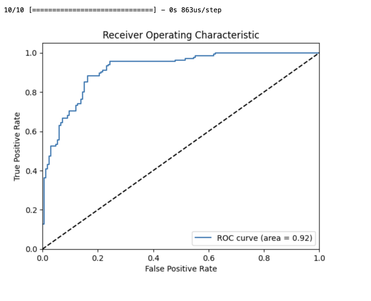
ROC-AUC evaluates the trade-off between the true positive and false positive rates across different threshold values. 

Other layers used in the architecture with their respective evaluation results. 

Layers	Test Accuracy	Train Accuracy	Precision	Recall	F1	ROC_AUC
[8] Single hidden layer	0.84	0.81	0.79	0.90	0.84	0.92
[12] Single hidden layer	0.85	0.81	0.79	0.90	0.84	0.92
[17] Single hidden layer	0.84	0.81	0.78	0.89	0.83	0.92
[16, 45] two hidden layers	0.84	0.81	0.79	0.89	0.83	0.92
[28, 23] two hidden layers	0.83	0.81	0.83	0.87	0.82	0.92
[35, 19] two hidden layers	0.82	0.81	0.82	0.88	0.82	0.92
[34, 21, 10] three hidden layers	0.83	0.81	0.83	0.87	0.82	0.92

From the above result, we can say that the single hidden layers had the best accuracy while the two hidden layers and 3 hidden layers had better precisions.  This suggests that the number of nodes can influence the accuracy of a model only to a certain limit. However, overly complex models are likely to overfit, highlighting the importance of striking a balance between generalisation and model complexity.

Furthermore, standardizing the features contributed to better convergence during training, indicating the significance of appropriate pre-processing steps.

Observation

• After several tries with this architecture and others, the accuracy value was between 85% and 81% with a loss of 0.34 +/- 1.5.

• Standardizing the features gave a better convergence while training the models, showing the significance of pre-processing techniques.

• Adding more hidden layers improved the evaluation metrics in certain instances, in others there was a slight reduction. One major disadvantage is that it is computationally expensive, requires more processing time, power, and memory.

• The number of nodes improved certain performance metrics, for instance the model’s precision increases when the nodes are increased. Although this led to a longer training time and in some cases, there was a slight decrease in performance especially with the Recall value.

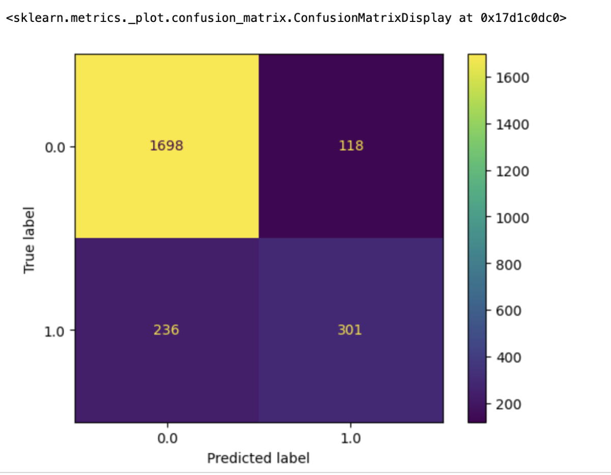
Confusion Matrix

Plot showing the best model’s accuracy and best model loss over different epochs. 

The Roc curve Area

Conclusion and Future Work:

This mini project involves a comprehensive analysis using a finance dataset to make binary classification and show how nodes and hidden layers affect ANN. Different nodes and hidden layers were tested and evaluated resulting in varying evaluation metrics. Future experiments can use other activation functions, regularisation techniques, or optimisation algorithms.

References:

Williams, G. (2023) The best time to buy everything | spending | U.S. news, The Best Time to Buy Everything. Available at: https://money.usnews.com/money/personal-finance/saving-and-budgeting/articles/the-best-time-of-year-to-buy-everything (Accessed: 14 May 2024). 

Kant, U. (2024) Complete guide to categorical features encoding guide, The Complete Guide to Encoding Categorical Features. Available at: https://kantschants.com/complete-guide-to-encoding-categorical-features (Accessed: 14 May 2024). 

Simon Benavides Pinjosovsky, P. (2023) Normalize data before or after split of training and testing data?, Medium. Available at: https://medium.com/@spinjosovsky/normalize-data-before-or-after-split-of-training-and-testing-data-7b8005f81e26#:~:text=The%20recommended%20approach%20is%20to,results%20and%20unrealistic%20performance%20evaluations. (Accessed: 27 May 2024).

Topper, N. (2023) Sigmoid activation function: An introduction, Built In. Available at: https://builtin.com/machine-learning/sigmoid-activation-function (Accessed: 28 May 2024). 

Aswini., S. (2023) Relu and sigmoid activation functions in a neural network – shiksha online, shiksha. Available at: https://www.shiksha.com/online-courses/articles/relu-and-sigmoid-activation-function/ (Accessed: 28 May 2024).